- PyTorch 教程
- PyTorch - 主页
- PyTorch - 简介
- PyTorch - 安装
- 神经网络的数学构建模块
- PyTorch - 神经网络基础知识
- 机器学习的通用工作流程
- 机器学习与深度学习
- 实施第一个神经网络
- 神经网络到功能块
- PyTorch - 术语
- PyTorch - 加载数据
- PyTorch - 线性回归
- PyTorch - 卷积神经网络
- PyTorch - 循环神经网络
- PyTorch - 数据集
- PyTorch - 修道院简介
- 从头开始训练修道院
- PyTorch - 修道院中的特征提取
- PyTorch - 修道院的可视化
- 使用Convents进行序列处理
- PyTorch - 词嵌入
- PyTorch - 递归神经网络
- PyTorch 有用资源
- PyTorch - 快速指南
- PyTorch - 有用的资源
- PyTorch - 讨论
PyTorch - 线性回归
在本章中,我们将重点介绍使用 TensorFlow 实现线性回归的基本示例。逻辑回归或线性回归是一种用于分类离散类别的监督机器学习方法。本章的目标是建立一个模型,用户可以通过该模型预测预测变量与一个或多个自变量之间的关系。
这两个变量之间的关系被认为是线性的,即,如果 y 是因变量,x 被认为是自变量,那么两个变量的线性回归关系将如下所示:
Y = Ax+b
接下来,我们将设计一种线性回归算法,它使我们能够理解下面给出的两个重要概念 -
- 成本函数
- 梯度下降算法
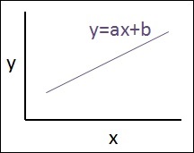
线性回归的示意图如下
解释结果
$$Y=ax+b$$
a的值为斜率。
b的值是y − 截距。
r是相关系数。
r 2是相关系数。
线性回归方程的图形视图如下 -
以下步骤用于使用 PyTorch 实现线性回归 -
步骤1
使用以下代码导入在 PyTorch 中创建线性回归所需的包 -
import numpy as np
import matplotlib.pyplot as plt
from matplotlib.animation import FuncAnimation
import seaborn as sns
import pandas as pd
%matplotlib inline

sns.set_style(style = 'whitegrid')
plt.rcParams["patch.force_edgecolor"] = True
第2步
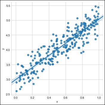
使用可用数据集创建单个训练集,如下所示 -
m = 2 # slope
c = 3 # interceptm = 2 # slope
c = 3 # intercept
x = np.random.rand(256)

noise = np.random.randn(256) / 4

y = x * m + c + noise

df = pd.DataFrame()
df['x'] = x
df['y'] = y

sns.lmplot(x ='x', y ='y', data = df)
步骤3
使用 PyTorch 库实现线性回归,如下所述 -
import torch
import torch.nn as nn
from torch.autograd import Variable
x_train = x.reshape(-1, 1).astype('float32')
y_train = y.reshape(-1, 1).astype('float32')
class LinearRegressionModel(nn.Module):
def __init__(self, input_dim, output_dim):
super(LinearRegressionModel, self).__init__()
self.linear = nn.Linear(input_dim, output_dim)
def forward(self, x):
out = self.linear(x)
return out
input_dim = x_train.shape[1]
output_dim = y_train.shape[1]
input_dim, output_dim(1, 1)
model = LinearRegressionModel(input_dim, output_dim)
criterion = nn.MSELoss()
[w, b] = model.parameters()
def get_param_values():
return w.data[0][0], b.data[0]
def plot_current_fit(title = ""):
plt.figure(figsize = (12,4))
plt.title(title)
plt.scatter(x, y, s = 8)
w1 = w.data[0][0]
b1 = b.data[0]
x1 = np.array([0., 1.])
y1 = x1 * w1 + b1
plt.plot(x1, y1, 'r', label = 'Current Fit ({:.3f}, {:.3f})'.format(w1, b1))
plt.xlabel('x (input)')
plt.ylabel('y (target)')
plt.legend()
plt.show()
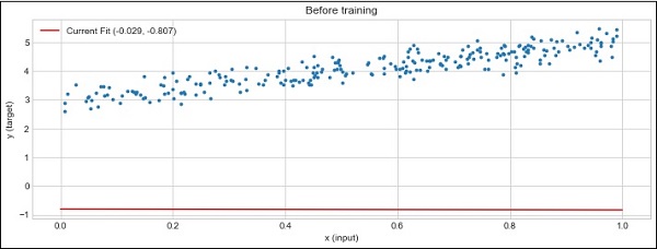
plot_current_fit('Before training')
生成的图如下 -